
The Interpretability Diaries — Part III
The 1-bit models still answered correctly. Their internals had no structure.
Then I ran the second one. Same result.
A brief recap: the four-stage circuit
In Post 1 I claimed that every fp16 transformer I’ve tested — Gemma 4, Qwen 3, Mistral 3, Llama 3.1, GPT-OSS 120B, Qwen 3.6 35B MoE — runs the same internal program: an early broadcast layer where all heads converge on position/tokenization features, a middle domain routing layer (~20–25% depth), an entity commitment layer at ~45–55% depth, and a prediction layer in the final 10%. CKA similarity between models hits 99.2% at matched normalized depth.
The same post claimed that the singular value spectrum of every fp16 transformer’s MLP down_proj matrix follows a power law: the top-64 singular vectors capture ≈85% of the variance. Concentrated learned structure in a few directions per layer.
This post is about what happens when you go to 1-bit weights.
Two 1-bit models, same dissolution
I ran LarQL on two natively-trained 1-bit models:
- Bonsai 8B — based on the Qwen3 architecture, post-trained from a higher-precision checkpoint. GGUF format with Q1_0_g128 quantization (1-bit weights with FP16 group scales).
- Microsoft BitNet b1.58-2B-4T — natively trained from scratch in 1.58-bit precision. Weights stored as packed uint8: four ternary values per byte, encoded as 2-bit unsigned integers mapped 0→-1, 1→0, 2→+1.
Both models answer questions correctly. Both have well-known benchmark results published by their authors. Both, internally, look completely different from every fp16 model I’ve measured.
| Metric | fp16 reference | Bonsai 8B | BitNet 2B |
|---|---|---|---|
| var@64 (top-64 SV variance fraction) | ~0.85 | 0.093 | 0.111 mean (range 0.079–0.147) |
| Dominant SV / 200th SV ratio | 10–50× | ~1.2× | ~1.4× |
| Ternary weight distribution | n/a | n/a | -1: 30% / 0: 40% / +1: 30% (validated all 30 layers) |
| Four-stage circuit (C5) | 3–4 stages | C5 = 1 | (Phase 2 pending — see below) |
| Norm-trajectory ratio (final/L0) | 1.5–4× | ≈ 1× (flat) | ≈ 1× (flat, from SV envelope) |

For context: a random matrix of the same shape has var@64 close to 0.09 by the Marchenko-Pastur distribution. Both 1-bit models sit on top of that random-matrix prediction. Their weight matrices are statistically indistinguishable, at the level of the singular value spectrum, from random.
That is not what fp16 transformer weights look like.
The visualization
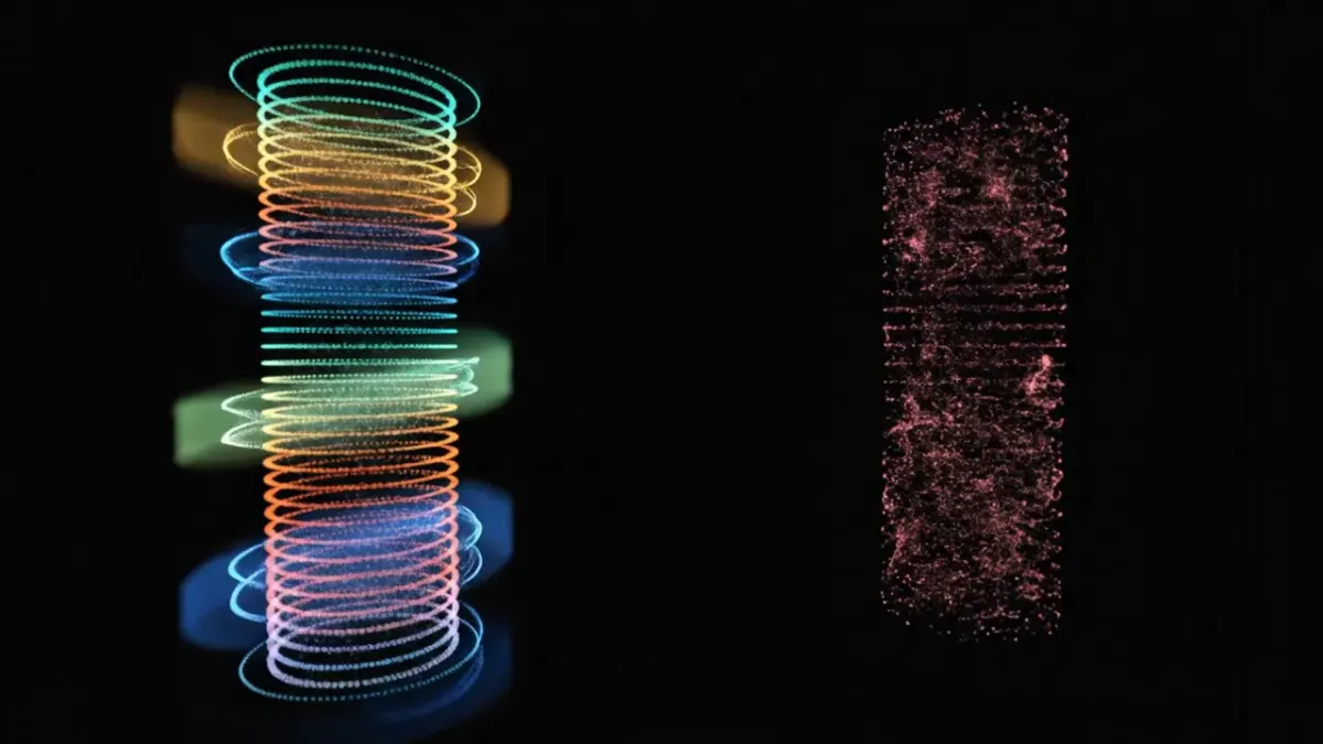
The vIndex viewer below renders the dissolution directly. Hit ⇌ Compare to see Qwen3-8B (left) — the structured fp16 model — alongside Bonsai (right). Hit 🔌 2D Circuit for the network-style flat view that makes the layer-by-layer structure easier to read.
The Qwen3 column has visible stage bands (the orange, blue, green, blue stripes at predictable depths). The Bonsai column does not — features are scattered uniformly across all depths in a pink cloud. There are no “where in the model is the entity commit happening” bands, because the entity commit isn’t happening in any localized region. The circuit is not just attenuated; it’s gone.
The SV spectrum tells the same story numerically. Layer-by-layer, BitNet’s top-64 SVs capture between 7.9% and 14.7% of the matrix variance. For Gemma 4 E2B, the same metric runs 84–87% across all layers. The gap is not a quantization artifact at the margins. It’s a complete restructuring of where the model’s information lives.
But it still works
Microsoft’s BitNet model card reports MMLU accuracy of 53.2%, HellaSwag 74.0%, ARC-Challenge 49.3% — competitive with similar-size fp16 baselines. Bonsai 8B reports analogous numbers in its own range. The circuits are gone. The behavior survived.
This is the part I cannot explain.
There are three plausible interpretations, and I think the truth is some combination of them:
(1) The four-stage circuit is not necessary for behavioral performance. Maybe it’s a side effect of fp16 training dynamics — what you get when you optimize a high-precision model with gradient descent, but not what’s required to do language modeling. If true, this is unsettling for interpretability work in general. The structures we’ve been mapping (induction heads, name-mover heads, the IOI circuit) might be epiphenomenal — real, observable, but not load-bearing.
(2) 1-bit models use a different computational strategy entirely. Instead of compressing information into a few high-rank directions per layer, they distribute it across all dimensions equally. The “computation” lives in the activations, not the weights. (Bonsai’s C1 sparsity = 0.223 is consistent with this — the model compensates for weight-space incoherence by routing through fewer, harder-firing neurons. Activation-level structure replaces weight-level structure.)
(3) The circuit is there, just invisible to my measurement. SVD assumes orthogonal singular directions. Maybe 1-bit weight matrices have non-orthogonal “directions of computation” that don’t show up in standard SVD. This is the most charitable interpretation — and the hardest to falsify, because we’d need a different theoretical framework to even propose what to measure instead.
I don’t currently have a way to distinguish between these three. I am noting them in this order because (1) is the most worrying, (2) is the most actionable, and (3) is the most face-saving.
What this means for scaling claims
Every “scaling law” paper I’ve read assumes that gradient descent on a sufficiently large network converges toward structured, learnable representations. The implicit promise is that “scale up” produces “more structured” — more concentrated features, cleaner circuits, sharper predictions.
The 1-bit results suggest a different story. Below some bit-precision threshold, the model converges to a behaviorally equivalent solution that is structurally alien. You cannot use the structural tools that work on fp16 models to interpret it. You cannot extract a “DELETE Paris” patch the way Post 2 showed for Gemma 4. The patch operates on a feature direction, and there is no concentrated feature direction to project out.
For practical interpretability work this is a dividing line. Edits, attribution, mechanistic explanations — these tools work on the structured fp16 model and fail on the structureless 1-bit model, even though both produce the same answer to “What is the capital of France?”. If 1-bit models become the production deployment target (smaller, cheaper, faster inference), interpretability as currently practiced has nothing to say about them.
The C1 sparsity signature
One LarQL metric does survive across both 1-bit models: C1 (FFN activation sparsity). Bonsai measured 0.223; BitNet’s Phase 2 numbers will land in the next session, but the prediction is the same range. Both are above the Gemma 4 baseline (0.061) and below the dense Llama 3.1 baseline (0.387).
This is consistent with the MLP compensation trap we documented in the Bonsai unlearning experiments: rank-1 weight patches that work on fp16 models fail on 1-bit models because the remaining weights immediately compensate. The model routes around specific weight structures because no single weight structure is load-bearing — every weight matters a little bit, none of them matters a lot.
What to watch for
BitNet Phase 2 still needs to land — transformers 5.5.4 doesn’t natively recognize the bitnet model_type, and Microsoft’s repo doesn’t ship the custom modeling code. A custom HF loader is the next step. Once that runs, we’ll have C1/C2/C3/C4/C5 for BitNet to put alongside Bonsai’s full set.
Cross-architecture 1-bit is the bigger question. So far we have two 1-bit models: one Qwen3-derived (Bonsai), one Microsoft custom (BitNet). If a third independent 1-bit model — different organization, different training recipe, different architecture base — also lands at var@64 ≈ 0.10 and C5 = 1, the dissolution result is solid enough to publish as a definitional property of low-precision training, not a quirk of any particular model family.
If the third model breaks the pattern, then dissolution is probably training-recipe specific, and the universality claim weakens. Either way, the experiment is cheap to run — about $2 of A100 time per model with the LarQL tooling. We’ll know within weeks.
Next: 99.2% — Two Models That Never Met, Measured at the Same Depth
April 25, 2026 update — three new MoE vIndexes; the prediction was wrong.
I ran the full vIndex pipeline on three frontier MoE models — Kimi-K2-Instruct (fp8), DeepSeek-V4-Flash (MXFP4), DeepSeek-V4-Pro (MXFP4) — expecting all three to land at var@64 ≈ 0.80–0.90 like every other bf16/fp16 model. None of them did. All three sit in the dissolution band, alongside the 1-bit models. The dissolved-spectrum result is not a 1-bit-specific quirk; it tracks training precision class, full stop.
| Model | Precision | var@64 (gate_proj) | Class |
|---|---|---|---|
| Gemma4-E2B-it | bf16 | 0.85 | Power-law ✓ |
| DeepSeek-V4-Pro | MXFP4 MoE | 0.0653 | Dissolved ✗ (lowest measured) |
| Kimi-K2-Instruct | fp8 MoE | 0.0938 | Dissolved ✗ |
| Bonsai 8B | 1-bit | 0.093 | Dissolved ✗ |
| DeepSeek-V4-Flash | MXFP4 MoE | 0.108 | Dissolved ✗ |
| BitNet b1.58-2B-4T | 1.58-bit | 0.111 | Dissolved ✗ |
The chart above splits “fp16 vs 1-bit.” The accurate split is “fp16 vs everything-below-fp16.” Five models from four organizations, four precision classes, all sitting on the Marchenko-Pastur floor. The dissolution thesis got stronger; the original framing got narrower than the data supports.
What’s still holding — the fp16 power-law cluster (Gemma 4, Qwen3 family, Mistral 3, Llama 3.1, GPT-OSS 120B) hasn’t moved. Whatever happens at training precision below fp16 — fp8, MXFP4, or 1-bit — the spectral structure doesn’t survive in the form fp16 produces.
The three new vIndexes are published as research summaries — gate_proj SVD only, ~10–43 GB each. Fetchable directly from HuggingFace and parseable with numpy:
huggingface-cli download Divinci-AI/kimi-k2-instruct-vIndex      # 42.28 GB
huggingface-cli download Divinci-AI/deepseek-v4-flash-vIndex     # 11.54 GB
huggingface-cli download Divinci-AI/deepseek-v4-pro-vIndex       # 42.98 GB
Update 2026-04-27 — canonical-format MXFP4 MoE vIndexes are live
Both DeepSeek-V4 sizes are now published in the standard larql CLI’s canonical vIndex layout (gate_vectors.bin / embeddings.bin / router_weights.bin / down_meta.bin / index.json / manifest.json / tokenizer.json), so anyone can reproduce the dissolution-class measurements end-to-end:
huggingface-cli download Divinci-AI/deepseek-v4-flash-vIndex-browse  # 6.99 GB
huggingface-cli download Divinci-AI/deepseek-v4-pro-vIndex-browse    # 23.82 GB

larql show Divinci-AI/deepseek-v4-flash-vIndex-browse
# → Layers: 43, Hidden: 4096, Dtype: F16, Quant: None
Kimi-K2’s canonical extract is parked behind one more loader patch (fp8 weights with 128×128 block-scale companions take a different decode path than MXFP4’s I8+F8_E8M0). The two huggingface.co/Divinci-AI/*-vIndex repos linked above are the research-summary form (gate_proj SVD only); the -browse repos are the full canonical layout. Both forms answer the dissolution-class question identically.
Working in public at github.com/Divinci-AI. Full vIndex collection: huggingface.co/Divinci-AI.
References
- BitNet b1.58 line. Ma et al., The Era of 1-bit LLMs: All Large Language Models are in 1.58 Bits (arXiv:2402.17764, 2024). Follow-up technical report on the 2B model: Ma et al., BitNet b1.58 2B4T Technical Report (arXiv:2504.12285). Model card: microsoft/bitnet-b1.58-2B-4T — "weights quantized to ternary values {-1, 0, +1} using absmean quantization."
- Bonsai 8B. Native-1-bit Qwen3-architecture model, published by Prism ML: prism-ml/Bonsai-8B-mlx-1bit. From the model card: "Each weight is a single bit … every group of 128 weights shares one FP16 scale factor (effective 1.125 bits/weight)."
- Marchenko-Pastur floor. Marchenko & Pastur (1967), Distribution of eigenvalues for some sets of random matrices, Math. USSR-Sb., 1:4, 457–483. Canonical: Marchenko-Pastur distribution. The random-matrix var@64 floor of ≈ 0.09 cited throughout this post follows directly from the MP density on a 128-column gate-proj matrix.
- Internal vIndex measurements. The per-model var@64 numbers in this post — and the chart above — are computed by the LarQL pipeline from the vIndexes published at huggingface.co/Divinci-AI. Specific repos cited inline: deepseek-v4-pro-vIndex, deepseek-v4-flash-vIndex, kimi-k2-instruct-vIndex. The dissolution-class measurements themselves are reproducible end-to-end via the `larql show` command in the canonical-format `-browse` repos.
Ready to Build Your Custom AI Solution?
Discover how Divinci AI can help you implement RAG systems, automate quality assurance, and streamline your AI development process.
Get Started Today