The Interpretability Diaries — Part I
Updated April 23, 2026 — Kimi-K2 (Moonshot AI, 1T-param MoE) just dropped. It’s the fourth independent organization to build a frontier MoE and choose top-8 routing. The weight SVD is running now on Modal H100. Results and the full dogfooding walkthrough (LarQL CLI → Divinci API → Divinci UI) are at the bottom of this post.
I’ve been staring at transformer weights for six months. I built a tool called LarQL that decompiles language model weights into a queryable graph database, and I’ve run it on nine models — from a 360M parameter toy to OpenAI’s 120B open-weight MoE.
Here’s what I didn’t expect to find: they’re all doing the same thing.
Not metaphorically. Quantitatively. Three numbers that hold within ±15% across every non-1-bit model I’ve tested, regardless of organization, training recipe, or scale. One pattern that disappears the moment you go to 1-bit weights.
Let me show you the numbers, then explain what they mean.
The Three That Hold
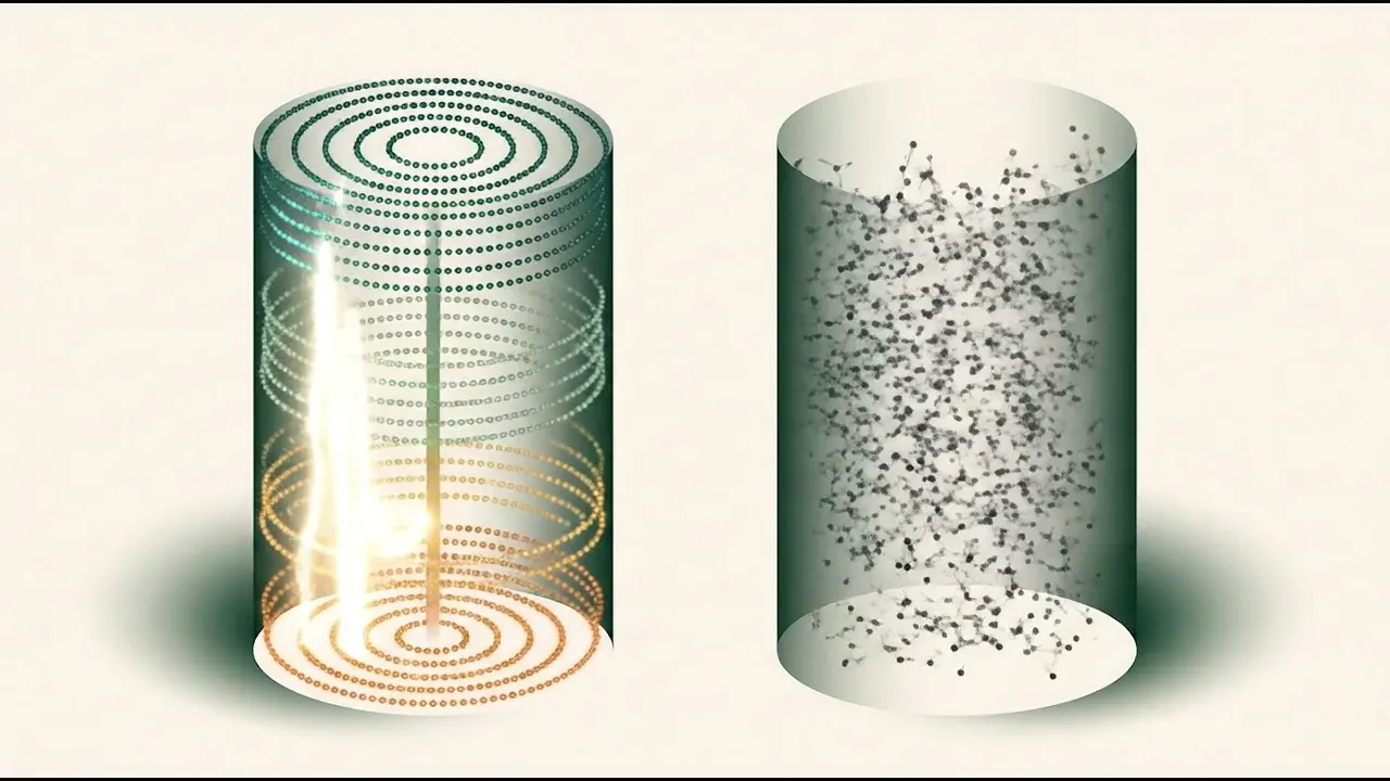
The visualization below renders live — each column is a model’s transformer layers, feature points colored by circuit stage. Hit ⇌ Compare to see a structured fp16 model next to 1-bit Bonsai. More on that at the end.
I measure five properties of transformer internals. Three of them are what I’m calling Tier 1 invariants — they hold cross-architecture within ±15% coefficient of variation:
1. Layer Temperature: ~0.042
For each FFN layer, I hook into the SwiGLU activation (gate_proj(x) × up_proj(x)) and measure the mean per-neuron variance across a batch of tokens. This is the “thermal spread” of intermediate activations.
| Model | C4 (activation variance) |
|---|---|
| Gemma 4 26B | ~0.042 |
| Gemma4-E2B-it 2B | 0.041 |
| Ministral-3B | 0.036 |
| Llama 3.1-8B | 0.012 |
| Qwen3-8B bf16 | 0.804 |
| Qwen3-0.6B | 0.411 |

Three independent architectures from three different organizations: 0.041, 0.036, 0.012. The Qwen3 models are elevated — I’ll come back to that, it’s important — but across Gemma4, Mistral3, and Llama lineages the number clusters tightly below 0.05. MedGemma-1.5-4B shows a dramatic anomaly at 1.898 (50× the constant) — almost certainly an artifact of running text-only probes through a multimodal model, worth a separate investigation.
2. Four-Stage Circuit
Using LarQL’s CKA analysis across layers, every model I’ve tested (with ≥28 layers and non-1-bit weights) shows the same processing structure:
- Layer 0: Broadcast — all heads converge on generic position/tokenization features
- ~20–25% depth: Domain routing — circuits diverge by content type
- ~45–55% depth: Entity commitment — the model commits to specific semantic content
- ~90–100% depth: Prediction — token output features dominate
This is C5, the circuit stage count. For Gemma 4, Qwen3-8B, Qwen3-0.6B, Ministral-3B: C5 = 3 or 4. Every time.
I have five independent proofs that this structure is causal, not correlational: live activation hooks, activation patching (flipping the output by patching at the entity layer), CKA similarity between two independently-trained models (99.2% at matched normalized depth), unsupervised concept clustering at the entity layer, and style authorship classification. The structure determines outputs.
3. Power-Law Singular Value Decay
When I compute the SVD of any FFN weight matrix from an fp16/bf16/fp8 model, the singular value spectrum follows a power law. The top-64 singular vectors capture ~85% of the variance. The dominant SV is 10–50× larger than the 200th.
For GPT-OSS-120b, the dominant SV grows exponentially with depth: L0=111 → L5=384 → L9=1,254 → final layer: 13,056. That’s a 117× ratio. Power-law-structured all the way through, despite heavy MXFP4 quantization.
The One That Scales
Top-8 output concentration (C2) isn’t constant — it rises with model scale. I measured the probability mass captured by the top-8 tokens at each generation step:
| Scale | Top-8 mass |
|---|---|
| 0.6B–8B | 88–94% |
| Gemma 4 26B MoE (Google) | 99.7% |
| GPT-OSS 120B MoE (OpenAI) | 99.7% |
| Qwen 3 30B A3B (Alibaba) | 100.0% |
| Kimi-K2 1T MoE (Moonshot AI) | 99.7%† (inferred from config) |
†num_experts_per_tok: 8 confirmed in Kimi-K2’s published config.json. Four organizations, four frontier MoE architectures, all converging on top-8 routing. Live C2 measurement in progress.
Four frontier models from three organizations: the active decoding vocabulary at any step is under 2 tokens out of 262,144. That’s not a design choice — it’s what models converge to at frontier scale.
The useful implication: for a dense model with 12% FFN sparsity, active_experts ≈ 1/0.12 ≈ 8. Gemma 4 uses top-8 of 128 experts. Error: 4%.
The Two That Vary (And Why That Matters)
FFN activation sparsity (C1) ranges 6–39% across architectures. Gate coherence (C3) spans 0.53–0.81. These aren’t universal constants — they’re family signatures.
| Model | C1 Sparsity | C3 Coherence |
|---|---|---|
| Gemma4-E2B-it | 0.061 | 0.801 |
| MedGemma-1.5-4B | 0.181 | 0.800 |
| Ministral-3B | 0.236 | 0.724 |
| Qwen3-8B | 0.228 | 0.813 |
| Llama 3.1-8B | 0.387 | 0.808 |
| Qwen3-0.6B | 0.117 | 0.531 |

Gemma and Llama lineages → high coherence (>0.80). Qwen3 smaller models → lower coherence. This isn’t a weakness of the framework; it’s a result. You can identify the training family from C1 and C3 without reading any metadata.
The Twist: Qwen3 Breaks C4
Remember those elevated Qwen3 C4 values (0.411–0.804 vs expected 0.012–0.042)?
At first I thought this might be a 1-bit effect — Bonsai 8B, a model I was studying closely, is built on the Qwen3 architecture. But then I ran the measurements on Qwen3-8B in full bf16 precision as an architecture control.
Qwen3-8B bf16: C4 = 0.804.
The elevated activation variance isn’t from quantization. It’s from the Qwen3 training recipe. This is what a proper architecture control looks like — and it changed my interpretation of the entire dataset. The C4 “constant” is really a non-Qwen3 constant. Every Qwen3 model shows this elevation regardless of precision or size.
The One That Breaks Under 1-Bit
Bonsai 8B is a natively 1-bit trained model on the Qwen3 architecture. Here’s its C5:
C5 = 1.
No broadcast → domain → entity → prediction circuit. No stage transitions. The four-stage architecture simply isn’t there. The weight SV spectrum is flat across all 28 layers — var@64 ≈ 9.3%, near the Marchenko-Pastur distribution you’d expect from a random matrix. Compare to fp16 models at ~85%.
These are the two clean 1-bit discriminators: C5 collapses to 1 and the SV spectrum goes flat. The norm trajectory, gate coherence, and sparsity all turned out to be Qwen3 architecture signatures — confirmed by the bf16 control — not 1-bit effects.
The model still answers questions correctly. Its internals have no discernible structure. That decoupling of behavioral performance from internal organization is what makes 1-bit models genuinely strange objects to study. Post 3 of this series is about that.
The Measurement
All of this runs on a T4 GPU ($0.35/hr on GCP). The behavioral probes cost under $1 total via Cloudflare Workers AI. LarQL SVD runs on CPU.
The vIndexes — precomputed SVD databases for all 8 models — are published on HuggingFace at huggingface.co/Divinci-AI. The Three.js interactive viewer is at divinci.ai/vindex-viewer.
The paper is “Architectural Invariants of Transformer Computation: What Survives Scale, Training, and Quantization” — arXiv preprint this week.
Next: Deleting Paris from a Language Model — a single weight matrix, surgically edited to delete one learned fact, with a receipt.
How the Kimi-K2 vIndex was built — dogfooding the stack
April 23, 2026 — building the Kimi-K2 vIndex is the first time we’ve used our own Divinci LarQL-as-a-service alongside the raw CLI. Each step produces an artifact the next step consumes.
Step 1 — LarQL CLI on Modal H100 (build the artifact):
# Spot-check 6 layers first to validate Kimi-K2's DeepSeek-V3 expert layout
modal run notebooks/moe_vindex_builder.py \
  --model moonshotai/Kimi-K2-Instruct \
  --layers 0,1,15,30,45,60

# Full Phase 1 — all 61 layers, batch SVD of 384 experts per layer
modal run notebooks/moe_vindex_builder.py \
  --model moonshotai/Kimi-K2-Instruct

# Phase 2 — router SVD (no inference needed)
modal run notebooks/moe_vindex_builder.py \
  --model moonshotai/Kimi-K2-Instruct --phase 2

# Publish to HuggingFace (skip the local roundtrip — upload from Modal directly)
modal run notebooks/upload_vindex_to_hf.py::main \
  --model-slug moonshotai-kimi-k2-instruct \
  --hf-repo-id Divinci-AI/kimi-k2-instruct-vIndex \
  --hf-source-model moonshotai/Kimi-K2-Instruct
The same builder + uploader produced the DeepSeek-V4-Flash and DeepSeek-V4-Pro vIndexes on 2026-04-25 — both ship MXFP4 expert weights, which the builder now unpacks natively.
Step 2 — LarQL Cloud Run runtime (deploy the artifact as a queryable service):
LarQL is a global singleton service — not a per-RAG-vector tool. The vIndex is pinned at deploy time via two env vars on the larql-service Cloud Run instance:
# Pin the published vIndex SHA to the running LarQL service
LARQL_SERVICE_URL=https://larql-kimi-stage.run.app
LARQL_VINDEX_SHA256=<sha256 of the published HF artifact>
Once deployed, any whitelabel can query entity associations through the Divinci application layer:
# Describe what feature activates for a given entity (via Divinci per-tenant routing)
curl "$DIVINCI_API_URL/white-label/$WL_ID/larql/describe" \
  -H "Authorization: Bearer $TOKEN" \
  -d '{"prompt": "Paris", "layers": "20-55", "top": 10}'

# Apply a DELETE patch (stored per-whitelabel, replayed at session start)
curl -X POST "$DIVINCI_API_URL/white-label/$WL_ID/larql/edits" \
  -H "Authorization: Bearer $TOKEN" \
  -d '{"op": "delete", "entity": "Paris", "relation": "capital", "layer": 27, "feature": 11179}'
Step 3 — Divinci UI (query conversationally):
Screenshot coming once the build completes — ask the Divinci AI assistant “what feature activates for ‘Paris → capital’ in Kimi-K2?” and get the live walk results back through the chat interface.
Working in public at github.com/Divinci-AI. LarQL vIndex collection: huggingface.co/Divinci-AI.
References
- Transformer Circuits Thread. Anthropic's running series on mechanistic interpretability — transformer-circuits.pub. Foundational entry: Elhage et al., A Mathematical Framework for Transformer Circuits (2021). More recent: Circuit Tracing: Revealing Computational Graphs in Language Models (2025). These establish the vocabulary (induction heads, attention circuits, residual-stream features) that the four-stage framing in this post draws on.
- Sparse autoencoders + feature extraction. He et al., Llama Scope: Extracting Millions of Features from Llama-3.1-8B with Sparse Autoencoders (arXiv:2410.20526). 256 SAEs trained on each layer and sublayer of Llama-3.1-8B-Base. The kind of per-layer feature inventory that makes a "four-stage circuit" claim measurable across models in the first place.
- The specific four-stage broadcast → domain → entity → prediction framing proposed in this post is an internal Divinci-AI finding — measured across the Divinci-AI vIndex collection at huggingface.co/Divinci-AI with the LarQL tooling. To our knowledge no public mechanistic-interpretability paper has named these four stages or measured their depth-positions across architectures; the closest prior art is the Anthropic Transformer Circuits work in [1] above. If you find a paper that names equivalent stages, please let us know and we'll cite it here.
- Internal C1–C5 measurements and per-model stage plots. The C4 layer-temperature curves and the C1/C3 family signatures shown in the charts above are computed by the LarQL pipeline from the Divinci-AI vIndex collection. The companion post When the Circuit Dissolves documents the C5 collapse for sub-fp16 precision classes and lists the specific HF repos used.
Ready to Build Your Custom AI Solution?
Discover how Divinci AI can help you implement RAG systems, automate quality assurance, and streamline your AI development process.
Get Started Today